
We are going to make reports with Excel Spreadsheets that will enable business owners and managers to compare their actual results for the current year with the same periods last year and also the current year’s budgeted figures. These reports will give early warnings should there be a downturn in business.

Monthly Management Accounts
My article Prepare A Business Budget emphasized the importance of forecasting your business performance for the next financial year. Taking time to complete an annual budget develops your full understanding of the business and market you are trading in. The budget provides a measure against which you can monitor your actual results on a month to month basis.
I am going to show you a format for producing your monthly management reports using Excel spreadsheets. The example I use refers to a business which provides printed and embroidered work wear and advertising clothing. The business purchases plain t-shirts, sweaters, tracksuits, caps etc. and then arranges for them to be printed or embroidered to the customers’ requirements. All figures reported are £’000’s.
Sample Page
Your monthly management reports will vary business to business. You may need reports on manufacturing performance; a report of sales, orders received and orders in hand for your product ranges; a report detailing the business overheads; a balance sheet; a trading and profit and loss account; a cash-flow statement and possibly some accounting ratios.
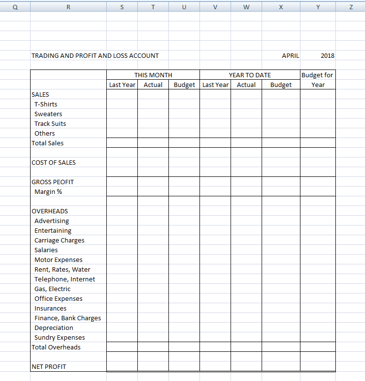
The report page I will prepare for this tuition is the Trading and Profit and Loss Account. Each month we will see the actual figures compared to the actual figures for the same month in the previous year and the figures that have been budgeted for the month. Further columns will show the cumulative figures for the financial year so far with those same comparisons. The final column shows the values that have been budgeted for the whole of the year.
Setting Up the Page Headings
To construct my report page I started at the spreadsheet cell S8 and typed Last Year, in cell T8 I typed Actual and in U8 I typed Budget. I then copied cells S8 through to U8 to cells V8,W8,X8. In cell Y7 I typed Budget for and in Y8 I typed Year. I centered the text in cell Y8.
At S7 I typed THIS MONTH and merge and centered this entry over the cells S7 to U7. I then typed YEAR TO DATE in V7 and merge and centered this entry over cells V7 to X7.
To complete my headings I typed TRADING AND PROFIT AND LOSS ACCOUNT in cell R5.
Page Content
In column R commencing R9 I entered the categories I want to report on and which are available from my accounting system. From here I have drawn the grid to provide the template as shown below. (The month and year will not be showing at this stage).
The Data Entry Area
The columns A through to P in our spreadsheet will become our data area. At cell A1 I entered the number 1, at A2 I entered the instruction which tells users to enter the period number they are working on or wish to view. In my case our financial year goes from April to March, so our first period is April and the number 1 in cell A1 will present us the figures for April. Our second period is May, the third June and so forth through to period 12 which is March.
Periods 1 to 9 (April to December) will be in (say) 2018 and periods 10 to 12 (January, February and March) will be in (say) 2019. My instruction at A4 requires these years to be entered at C4 and D4. To complete my headings in the data area I want to add the names for each period (the months) and I enter each month in capital letters starting with my first period APRIL in cell C5, MAY in D5, JUNE in E5 through to MARCH in N5. Each of these cells I have right aligned.
Next I copy the categories I entered in column R over to column B. I copy R9 through to R37 into my data area at B9 through to B37. On row 5 we have the month that each column relates to. We will be entering our data for April in column C, May in column D etc.
The Excel “Choose” Instruction
For more on the Choose function within Excel click here
Columns O and P will be used to choose the data according to the period number entered at A1.
At row 4 we have entry requirements for the (part) years included within our 12 months reporting. Our example has included 2018 (to cover April to December) and 2019 (for January to March). In cell O4 I have the formula: =IF($A$1<10,C4,D4) This is the formula if your financial year is April to March. The explanation of this formula in O4 is: if the number entered in cell A1 is less than 10, the value in cell C4 will be shown at O4. If the number at A1 is 10, 11 or 12 then the value in cell D4 will be shown at O4. Periods 1 to 9 are April to December and 2018 will show, periods 10 to 12 are January, February and March of the next year and 2019 will show.
We now want to do something similar to show the month being reported upon in cell O5. Whereas the year would be one of just two values, the month can be any one of twelve (APRIL, MAY, JUNE etc.). The function we use for the majority of our data is the CHOOSE function. Choose will use the index number at A1 (the period number) to select the month name or data we have used in columns C through to N.
To select the month according to the period number used at A1 we enter the following formula at cell O5: =CHOOSE($A$1,C5,D5,E5,F5,G5,H5,I5,J5,K5,L5,M5,N5)
If the period entered at A1 was 9 the cell accessed would be the ninth entry (starting at C5) which is K5 and the month at K5 is DECEMBER (the ninth month of our financial year) and that month will show at O5.
The month and year can now be added to our page heading. In cell X5 we enter =$O$5 and in cell Y5 the formula is =$O$4 I have aligned cell X5 to right-hand side and cell Y5 to left-hand side so that the month and year will be next to each other (no gaps) no matter how many letters are included in the month, 3 for May up to 9 for September. Adjust the widths of columns R to Y as needed to accommodate the longest wording.
Use of the $ Sign
The $ signs in the formulas prevent the column or row numbers changing when the cell is copied elsewhere in the spreadsheet. By putting a $ sign before the column and row references we can copy cells X5 and Y5 to anywhere else in our spreadsheet and it will give us the same Month and Year. The benefit here is, should we be preparing a number of pages we can just copy cells X5 and Y5 and we will have the month and year appearing in all of our headings.
Calculations in the Data Input Area
Back to the data area to complete lines 9 to 37. We want to calculate the totals on lines 14 and 35 and the Gross Profit, Gross Margin and Net Profit on lines 18, 19 and 37. Cell C14 will have the formula =SUM(C10:C13) and we will then copy that cell to D14 through to N14. Similarly cell C35 will be =SUM(C22:C34) The Gross Profit calculation at C18 is =C14-C16 and the Net Profit calculation at C37 is =C18-C35 The Gross Margin at C19 is the calculation =C18*100/C14 The calculations in lines 14, 18, 19, 35 and 37 will be copied to D through to N in each case. We now set the cells C19 through to P19 to two decimal places.
For the remainder of column O we can copy the cell at O5 to O10 through to O37 and then delete the entries of the lines not required – cells O15, O17, O20, O21 and O36.
It is good practice to protect those rows with calculations to avoid accidentally over-writing the formulas.
Using “Choose” in the Data Input Area
We are going to use column P to calculate the Year To Date figures. At P10 the calculation will be =CHOOSE($a$1,C10,SUM(C10:D10),SUM(C10:E10),SUM(C10:F10),SUM(C10:G10),SUM(C10:H10),SUM(C10:I10),SUM(C10:J10),SUM(C10:K10),SUM(C10:L10),SUM(C10:M10),SUM(C10:N10))
We now copy P10 to cells P11 through to P14, P16, P18, P22 through to P35 and P37. Our Gross Margin % cell at P19 will have the following calculation =P18*100/P14
It is good practice to protect the area O4 to P37.
Last Year and Budget Data Areas
I copied the area A9 to P37 into A509 to P537 which will be my data area for our Last Year figures, I copied the area again to A1009 to A1037 which will provide an area for our budget figures.
I have left an area of almost 500 lines between each so that we can add other report pages.
Finalizing the Reporting Page
In order to pick up the data into our Trading and Profit and Loss Account we enter the following in cells on line 10. The Month Actual at T10 will be =O10 This Month Last Year we add 500 to the cell line so S10 will be =O510 and This Month Budget we add a further 500 so U10 will be =O1010.
For the Year To Date the same applies but this time we pick up data from column P so Year To Date cells V10 will be =P510 W10 will be =P10 and X10 will be =P1010. We complete by calculating the Budget for Year at Y10 which will be the calculation =SUM(c1010:N1010)
Now copy S10 through to Y10 to rows 11 through to 37 and then delete that data from rows 15, 17, 20, 21 and 36. Row 19 change to two decimal places and cell Y19 change to Y18*100/Y14
Note that in copying you may have lost some grid lines so replace these and you are finished.
Looking Ahead
At the end of a year you can copy the data area of the current year (A9 to P37) to the last year area (A509:P537) and blank the input areas of C9 to N37 in readiness for the new year’s figures, keeping the lines with calculation formulas in the cells.
You can add additional report pages using columns A to P for the data but starting the new page layout further along the columns at column AA to accommodate different page layouts with different column widths.
Be aware, if you enter additional lines to a page you must add the line to the same place in the three areas, the current year, last year and budget.
You cannot delete a line whilst there is data in the last year section.
Should you have any comments or questions on this article, please leave them in the area below and I will be very pleased to respond.
Colin